Geometry Transformation Widget

The Geometry Transformation widget calculates \(G\)-vectors, azimuthal angles (\(\eta\)), and reciprocal distances (\(ds\)) from spatially corrected 3D peaks. It allows for real-time validation of geometry parameters against theoretical lattice rings.

Functionality

This widget is used for:

1. Geometry Parameterization: Manually editing or loading .par or .json or .poni file to define the experimental setup (distance, tilt, etc.).

2. Lattice Overlay: Providing a theoretical visual guide by plotting diffraction rings based on unit cell parameters.

3. Custom visualization: Visualizing calculated peaks with standard axes (\(ds\) vs \(\eta\)) and custom user-defined ones.

User Interface

Control Panel

The left panel contains the configuration and execution logic.

Geometry Settings

This section defines the physical spatial relationship between the sample and the detector. You can configure these parameters using one of the two methods below.

1. Import from File: Loading a pre-calibrated file will automatically populate the manual entry fields.

   • .par: ImageD11 geometry parameter files.

   • .json: Standard JSON configuration files.

   • .poni: PyFAI “Point Of Normal Incidence” calibration files.

2. Editable Parameters: A collapsible group where you can define:

   • Distance: Sample-to-detector distance \(\mu\).

   • Wavelength: Beam wavelength \(\AA\).

   • Tilts (\(x, y, z\)): Detector orientation angles in radians.

   • Centers (\(y, z\)): Direct beam intersection coordinates on the detector.

Attention

Important: The parameters listed above are a subset of the full internal geometry model.

While these are the most commonly adjusted fields, other fixed parameters (such as pixel sizes or detector alignment corrections) may be inherited from the loaded calibration file or provided as default values in the gui.

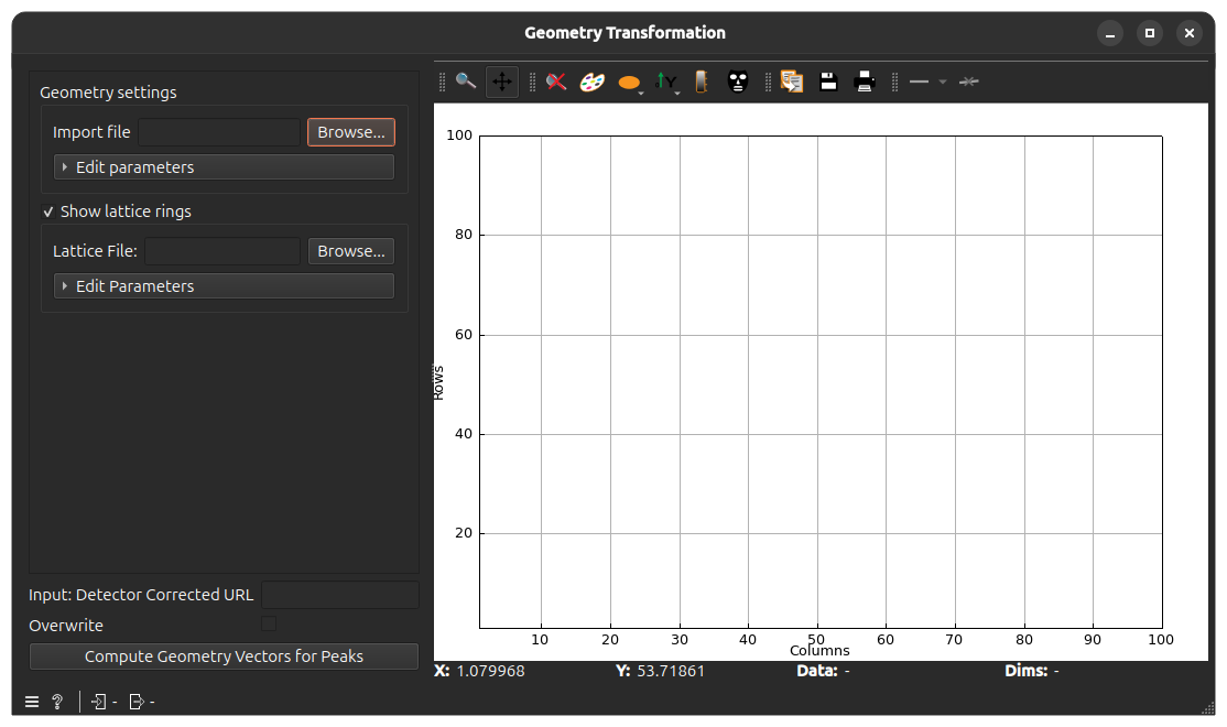
Lattice Settings

Used for visual validation of the geometry.

Supported Lattice File Formats:

• .par: Standard ImageD11 parameter files.

• .cif: Crystallographic Information File files.

Or you can manually edit:

• Lattice Parameters: Input for the three lengths \(a, b, c\) and the three angles \(\alpha, \beta, \gamma\) of the lattice unit cell.

• Space Group: Symmetry setting to calculate allowed reflections (number format).

• Show Rings: Toggles the overlay of theoretical diffraction rings on the plot.

Execution Control

• Compute Geometry Vectors: Generates the \(G\)-vectors for the spotted peaks.

• Overwrite: If checked, existing Nexus groups for geometry-updated peaks will be replaced.

Main View (Tabs)

The right side provides two distinct views of the data.

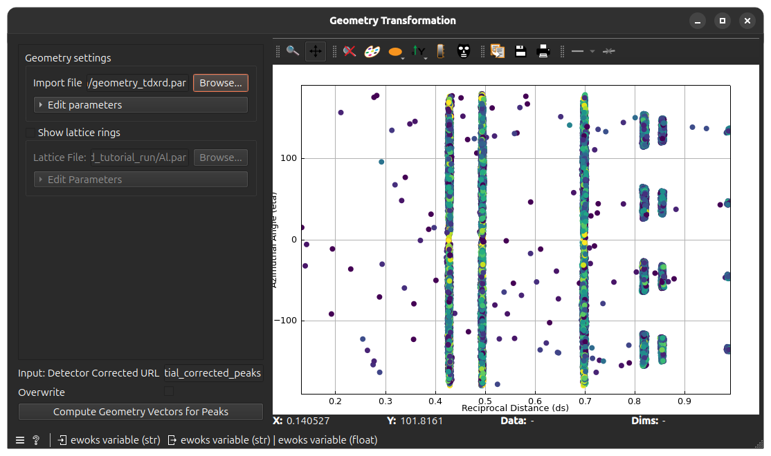
1. G-Vector Peaks Tab

Displays the primary result of the transformation.

• X-Axis: Reciprocal distance (\(ds\)).

• Y-Axis: Azimuthal angle (\(\eta\)).

• Color Map: Logarithmic scaling of peak intensity (Number of pixels).

• Overlay: Theoretical rings (if Lattice Settings are enabled) appear as vertical markers to verify if the experimental \(ds\) peaks align with expected crystal reflections.

2. Custom Peak Analysis Tab

Utilizes the user editable xy-axis peaks attributes to allow for arbitrary data exploration.

• Axis Selection: Users can choose any attribute from the 3D peaks (e.g., intensity, omega, ds, G_x) to plot against another.

Example Usage

1. Connect a widget that outputs a detector_corrected_url or browse from your folder and select the detector corrected data group.

2. Select your geometry .par file in the GeometryControlBox.

3. Optional: Select your reference lattice .par file in the LatticeBox

4. Click Execute. The plot will show \(ds\) vs \(\eta\) plot corresponding to the generated \(G\)-vectors.