Run a 3DXRD workflow#
Get started#
To check the different options to install and start processing 3DXRD in graphical user interface kindly follow the Installation page.
Then, open the Orange canvas by running
ewoks-canvas
The typical 3DXRD workflow can then be opened by navigation to Help > Example workflows. You will get the following workflow
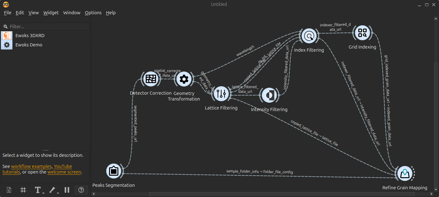
Attention
From now on, remember to save regularly your workflow!
Peak segmentation#
The first step of the workflow is to extract diffraction peaks from the raw data, a process known as segmentation.
Loading Data#
Double-click the Peaks segmentation node to open the widget.
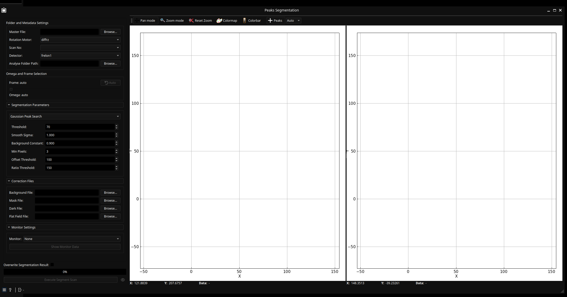
Select Master File: At the top-left, click Browse to select the Bliss master file containing your 3DXRD data.
Auto-Configuration: Once loaded, the widget automatically detects motor and detector names. If a dropdown has only one valid option, it will be disabled to prevent errors.
Analyse Folder: You can modify the Analyse Folder Path where the segmented output files will be stored.
Configuring the Segmenter#
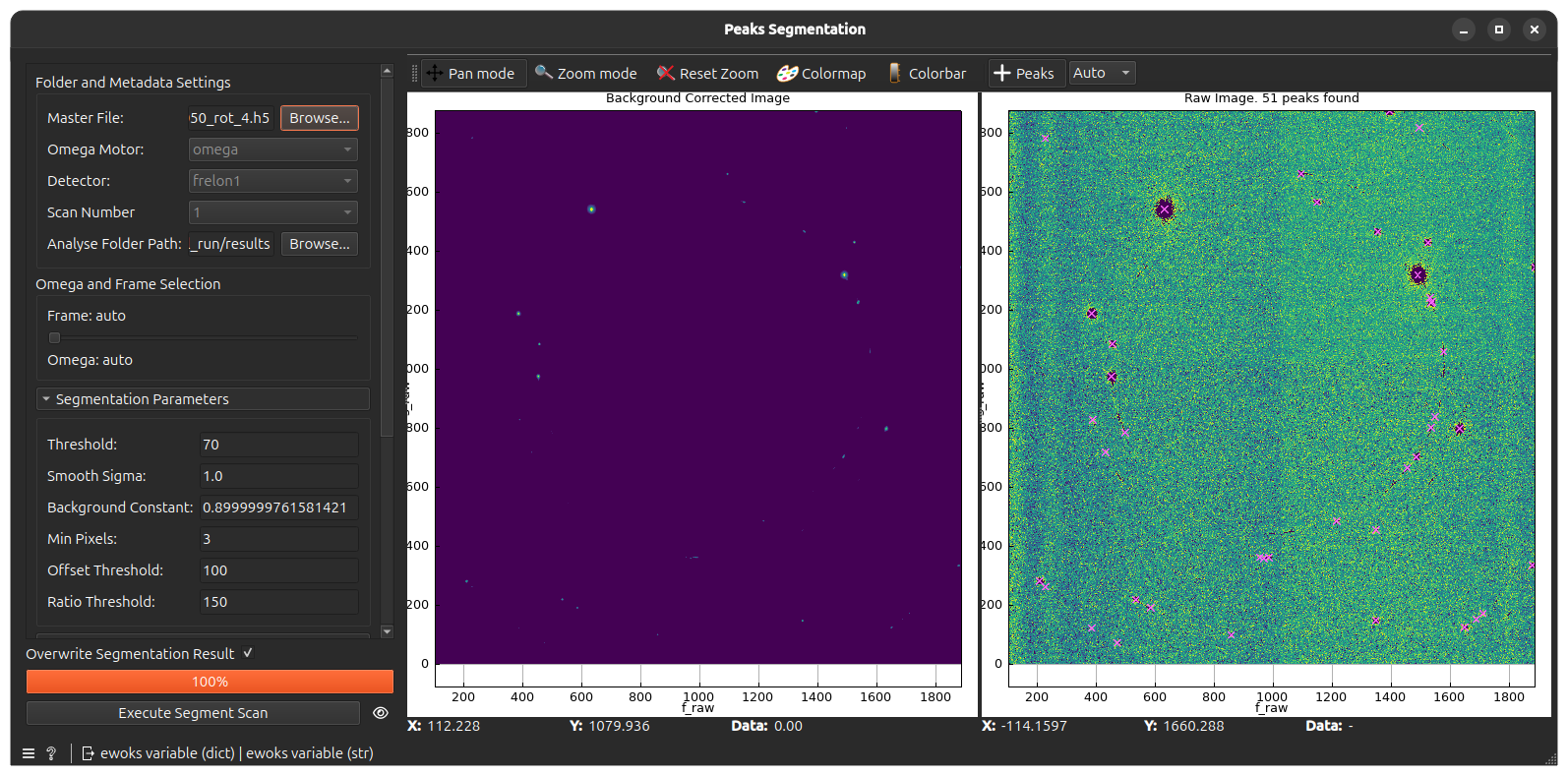
The widget provides a real-time preview of the segmentation for a single frame.
Visual Feedback: The left panel shows the background-corrected image; the right panel shows the raw image with markers indicating detected peaks.
Algorithm Selection: By default, the widget uses the Gaussian Peak Search algorithm. You can change the algorithm via the dropdown in the Segmentation Parameters box. Changing the algorithm will automatically update the settings box with relevant parameters.
Tip
If you are unsure about a parameter, hover over the field to see a detailed hint.
Frame Selection and Tuning#
Frame Selection: The widget initially targets the frame with the highest intensity (Frame: auto). Use the slider in the Omega and frame selection section to choose a specific frame index. The corresponding omega value will be displayed next to the slider.
Live Updates: Any change to parameters in the Segmentation Parameters or Correction files sections will automatically re-trigger the segmentation for the current preview frame.
Validating segmentation#
Now, the aim is to find the right segmentation parameters for your sample. For this, change the parameters and observe how the detected peak positions evolve.
Ideally, you should get something like this:
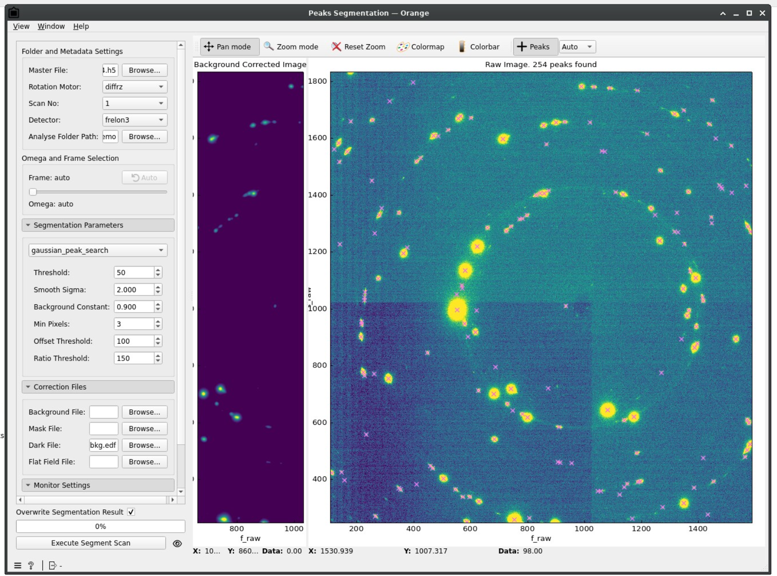
Namely:
✅ Detected peaks are centered on diffraction spots
✅ No peaks are detected outside of diffraction spots
✅ One-to-one correspondance with detected peaks and diffraction spots
For comparison, we show here an example where segmentation parameters are not adapted:
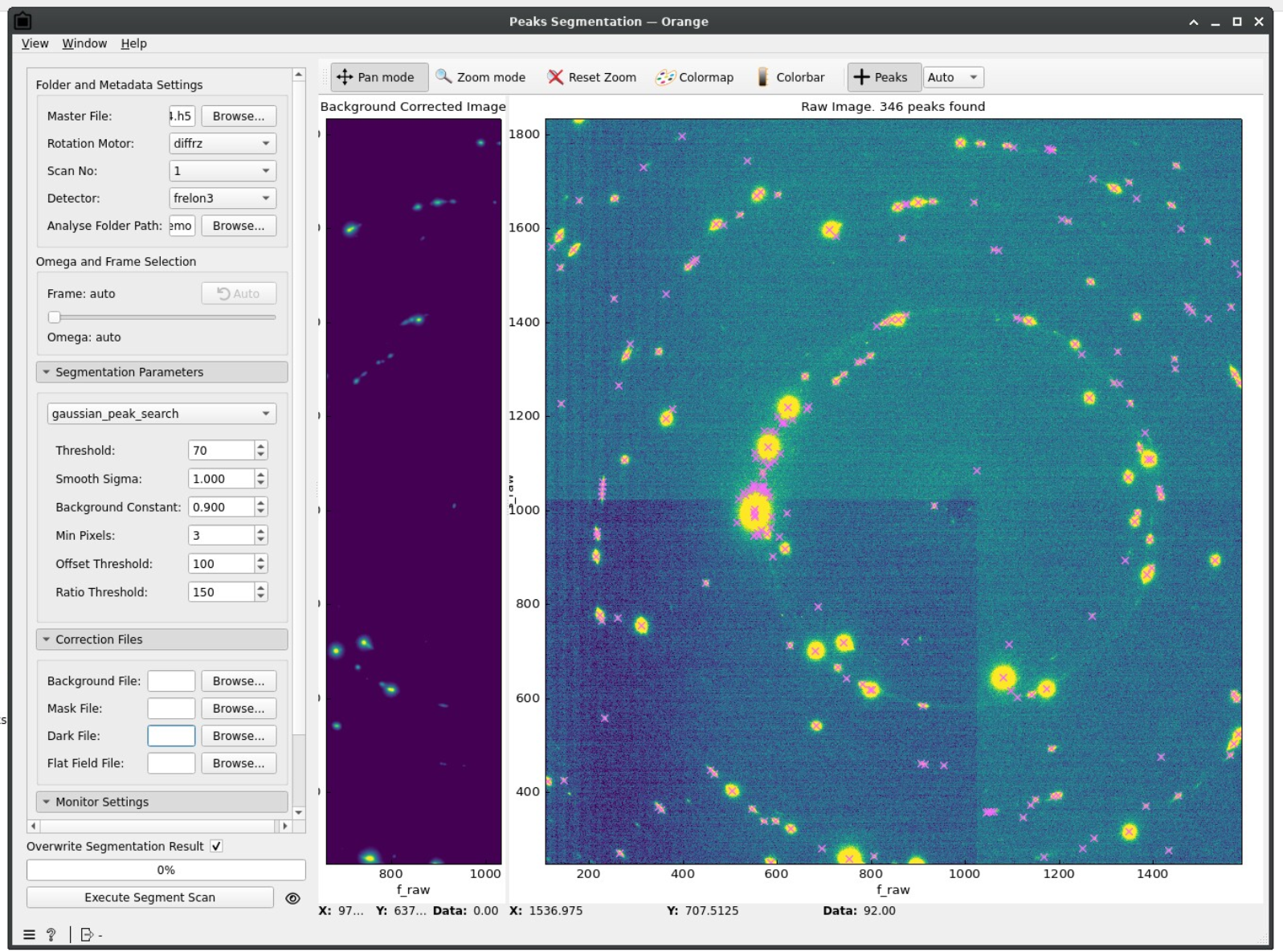
Namely:
❌ Multiple peaks are detected for one diffraction spot
❌ Detected peaks are mislaligned with respect to the diffraction spot
❌ Peaks are detected although there is no corresponding diffraction spot
Executing Full Scan#
Once the parameters are tuned for a single frame, click Execute Segment Scan to process the entire stack.
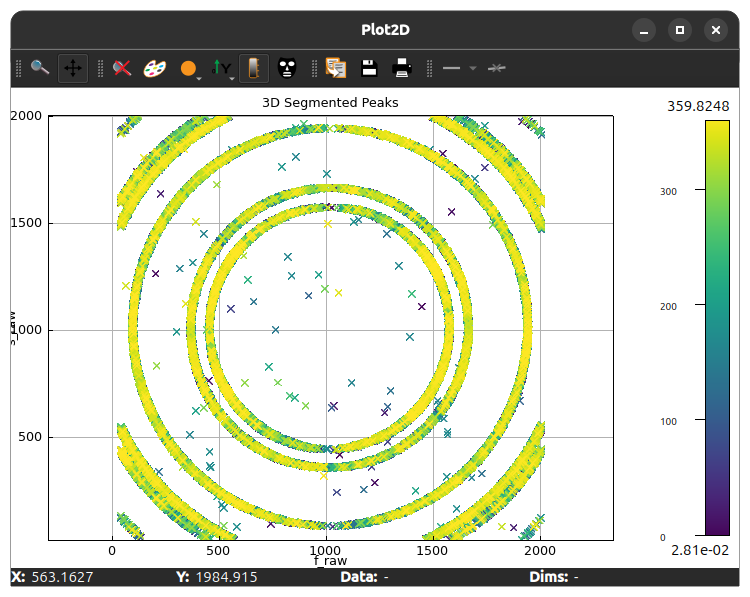
While the scan is running, the widget will be disabled and a progress bar will indicate the status. Upon completion, a window will display the positions of all segmented peaks, color-coded by their omega rotation angle.
Note
While not mandatory, it is possible to renormalize frame intensities during the full segmentation. For this, provide the name of the monitor dataset via the Monitor dropdown.
The monitor data can be inspected by clicking Show Monitor Data.
The progress bar at the bottom will show the progress of the segmentation. Once the segmentation is complete, you will get a pop-up with a plot showing the full segmentation results
Tip
If you closed the window showing the full segmentation results, you can show it again by clicking on the 👁️ button near the Execute Segment Scan.
These results are automatically saved in a HDF5 file located in the analysis folder chosen above, in a subfolder that will depend on the Bliss sample and dataset name, mirroring the RAW_DATA structure. See the Data format page for more information.
All tasks results will be saved in this output file inside different groups. Segmented results will be saved under the group <scan_number>/segmented_3d_peaks.
If you are happy with the result, you can move to the next widget Detector correction.
Else, change the parameters, inspect the results for single frame (see Validating segmentation above) and re-run the segmentation until it is satisfactory. The Overwrite Segmentation Result will have to be checked to overwrite previous results contained in the group segmented_3d_peaks of the output file.
Detector correction#
Real detector modules are not completely flat and this can lead to errors in the estimation of the coordinates of peaks in the reciprocal space. The aim of the Detector correction is to correct those errors.
Double-click on the Detector correction node, you will get the following window
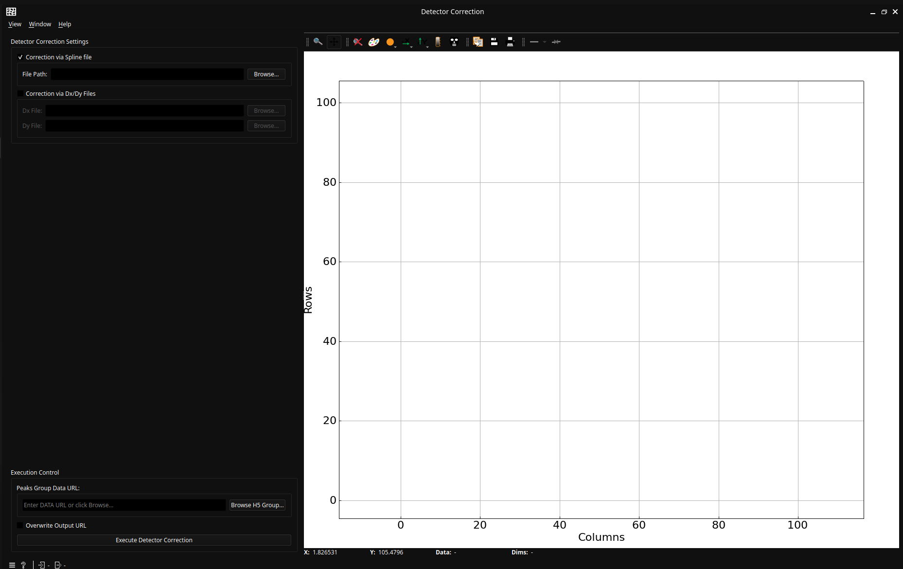
On the left, you can choose between a correction using a Spline file or two e2dx/e2dy files. Pick the appropriate one and load the correction file(s) via the corresponding Browse button(s).
Click then on Execute detector correction. The plot on the right will update with two different set of points:
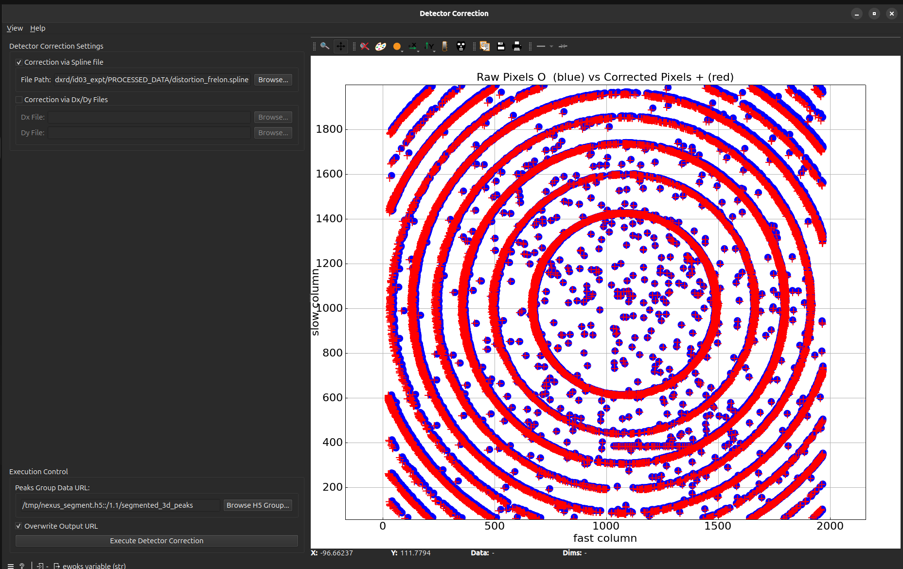
The first set of points (blue points in the picture) correspond to the uncorrected peak positions from the previous Peaks Segmentation task while the second set (red crosses in the picture) correspond to the corrected peak positions according to the loaded detector correction files. The plot therefore allows to visualize the effect of the detector correction.
The results will be saved in the scan group of the output file under spatial_corrected_peaks.
The following tasks will use the corrected peaks positions.
Geometry transformation#
The peaks positions are given in the detector frame of reference. For further data treatment, it is needed to project the positions in the lab frame of reference. For this, you have to supply geometric parameters describing your setup in the Geometry transformation widget.
Double-click on the Geometry transformation node, you will get the following window
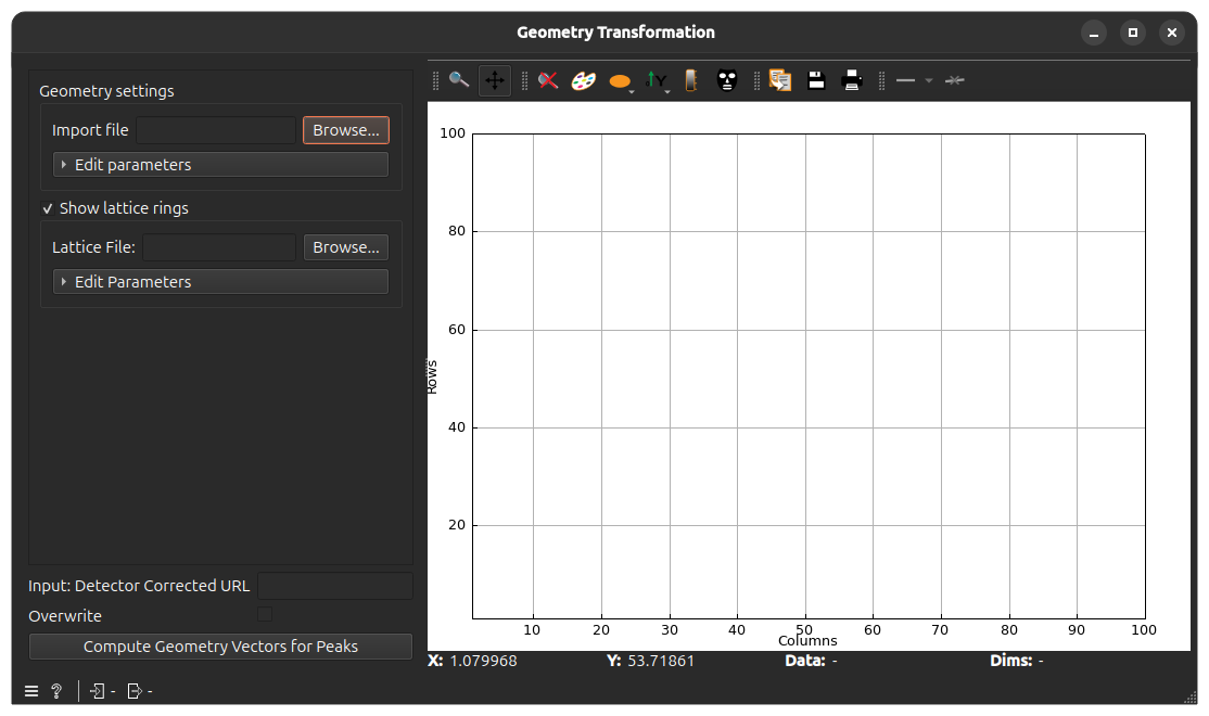
To supply the parameters, load the .par file obtained from calibration by clicking on Browse on the top-left Geometry settings section.
Once the geometry parameters are set, click on Compute Geometry Vectors for Peaks. The plot on the right will then show the computed azimuthal angle vs. reciprocal distance of all peaks.
The results will be saved in the scan group of the output file under spatial_corrected_peaks.
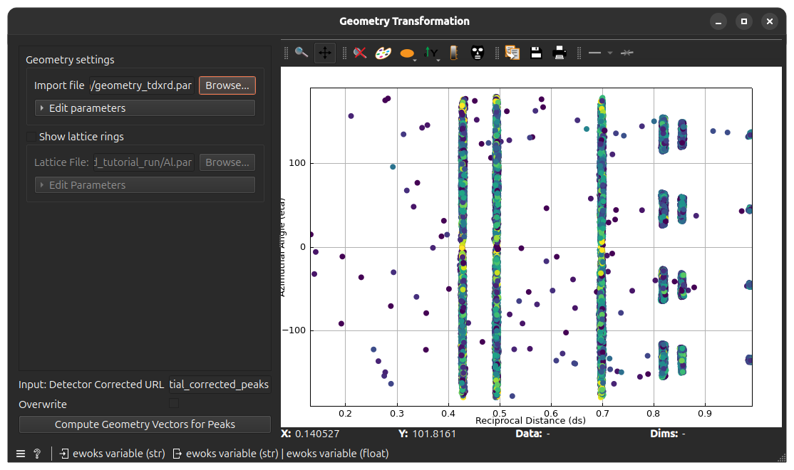
If the geometry was well parametrized, peaks should be more or less grouped in vertical lines that correspond to the diffraction rings.
To help diagnosis, you can load a file containing the expected lattice parameters. For this, check the Show lattice rings checkbox and click Browse to load a .par or .cif file (see File formats). The corresponding lattice rings will appear on the plot as colored vertical lines.
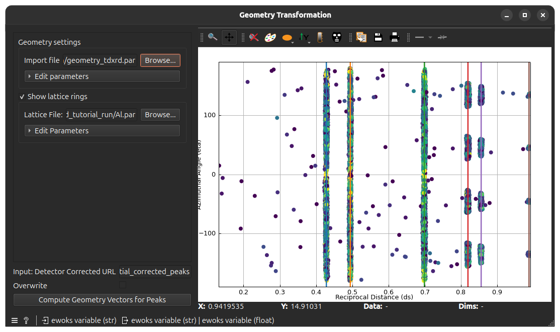
If the peaks positions match the lattice rings (as shown on the screenshot above), you can move to the next widget.
Warning
If this is not the case, you can edit the geometry parameters manually by clicking on Edit parameters in the Geometry settings group. Remember to check Overwrite to overwrite the previous results contained in the output file.
But the best thing would be to redo a calibration to produce a new .par file.
Filtering#
Attention
Did you save your workflow?
By opening a saved workflow, you can resume working at the last executed task.
Before moving to Indexing (i.e. attributing peaks to grains), it is essential to filter the peaks found by the segmentation steps to keep only the ones that are relevant. The filtering goes through three steps:
Lattice filtering: keep only peaks that are close to the expected peaks for a given lattice. A lattice file needs to be provided.
Intensity filtering: keep only a fraction of peaks to keep based on intensity.
Index filtering: same as lattice filtering but ring indices must be provided to keep only the peaks close to those rings.
All these widgets operate according the same principle: some peaks are given as input, the task filters some of them and returns the peaks that will be kept for the next operations.
Lattice filtering#
Double-click on the Lattice Filtering node, you will get the following window
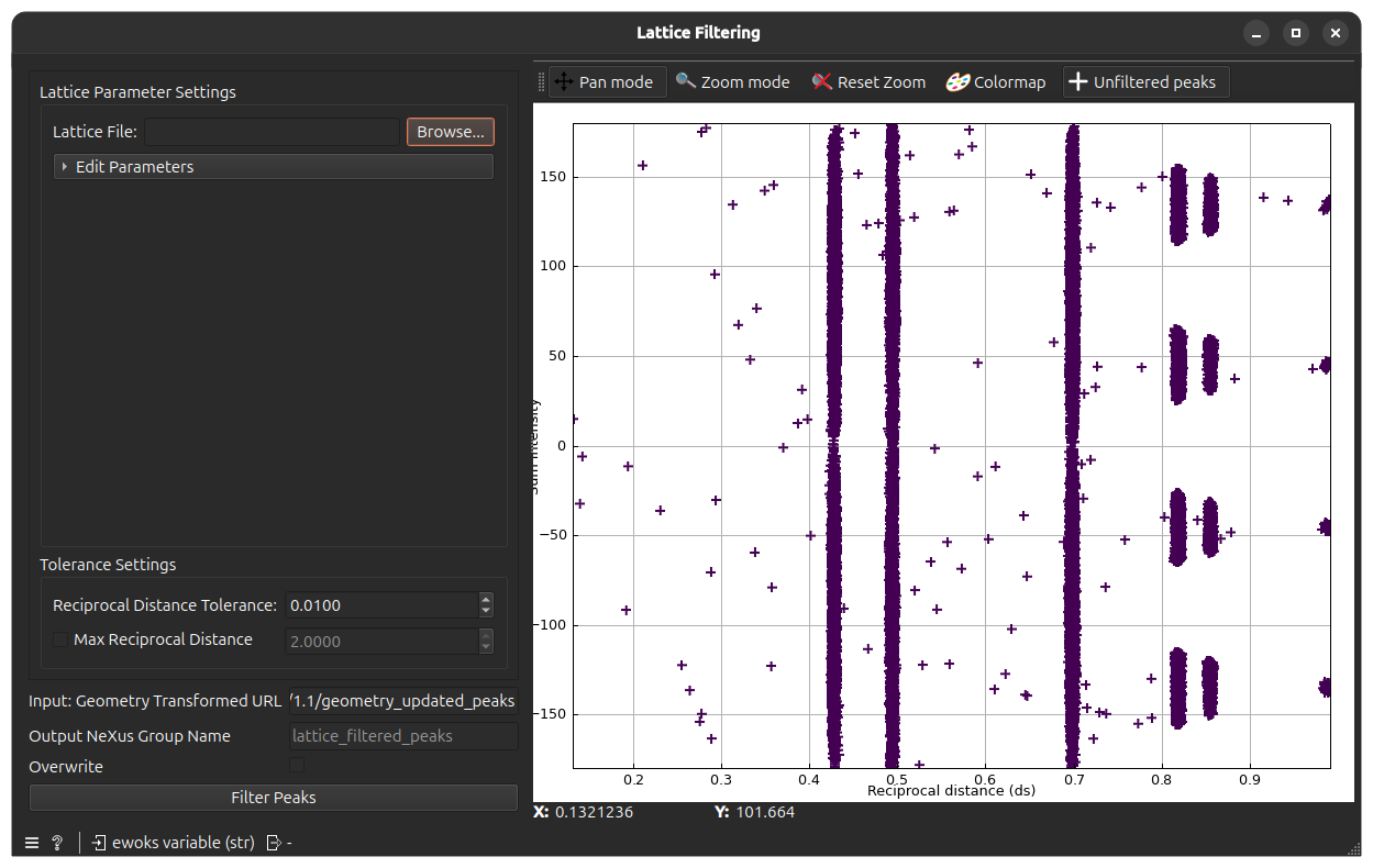
The peaks from the previously run Geometry Transformation task will be displayed as crosses on the plot (displayed again as computed azimuthal angle vs. reciprocal distance). These are the input or unfiltered peaks.
The aim of the widget is to keep only the peaks that are close a lattice ring. This allows to discard peaks that do not have crystallographic meaning.
For this, you have to load a lattice file corresponding to the expected lattice of the sample grains. Click Browse on the top-left and chose a .par or .cif file containing the lattice parameters.
Once this is done, lattice rings will be shown as colored lines on the plot. Click now Filter Peaks to start filtering according to these rings.
After task completion, the peaks that will be kept will appear as round markers.
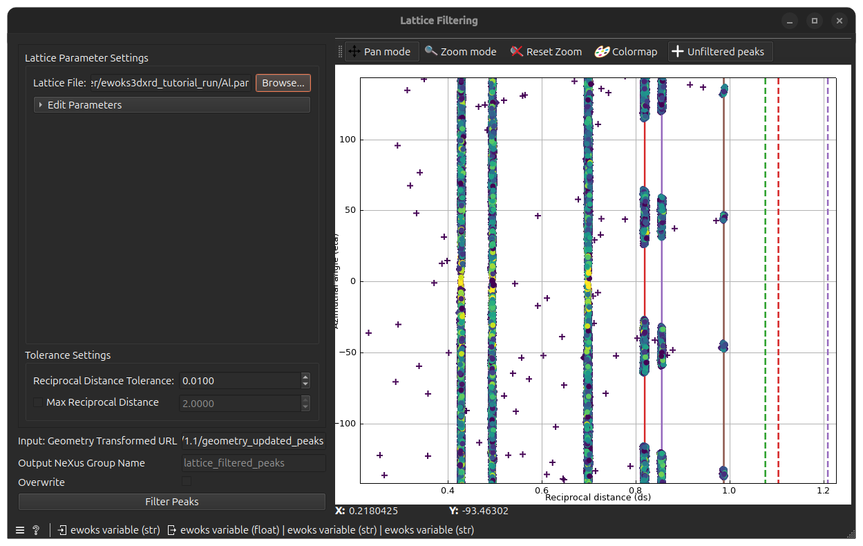
You can now check if all the relevant peaks are kept. If not, tune the Tolerance Settings below:
Reciprocal Distance Tolerance: this is the maximum distance between a peak and a ring for the peak to be kept. Increasing it makes the filtering more tolerant (more peaks are kept).
Max Reciprocal Distance: this is an optional cutoff value. If the checkbox is checked, all peaks above this reciprocal distance will be discarded.
As usual, remember to check Overwrite if you run the task once again. You can also choose to change the Output NeXus Group Name to save the peaks in a different group name (default: lattice_filtered_peaks).
Intensity filtering#
Double-click on the Intensity Filtering node, you will get the following window
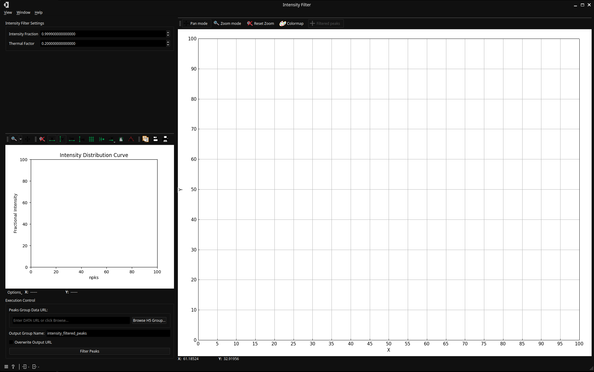
Again, the peaks from the previous task (Lattice Filtering) will be displayed as crosses on the plot. But this time, the plot is showing the intensity of the peaks against the reciprocal distance.
This widget allows to filter a fraction of the peaks to keep only the ones with the highest intensity.
By default, the Intensity Fraction parameter is set to 1.0 so that all peaks are kept. Low-intensity peaks can be discarded by reducing this value
For example, 0.5 will only discard half the peaks, keeping the ones with highest intensity. But usually, the fraction should be between 0.95 and 0.99 depending on the dataset.
By clicking on Filter Peaks, the results will be saved in the output file and the plot will be updated as kept peaks will be appear as round markers.
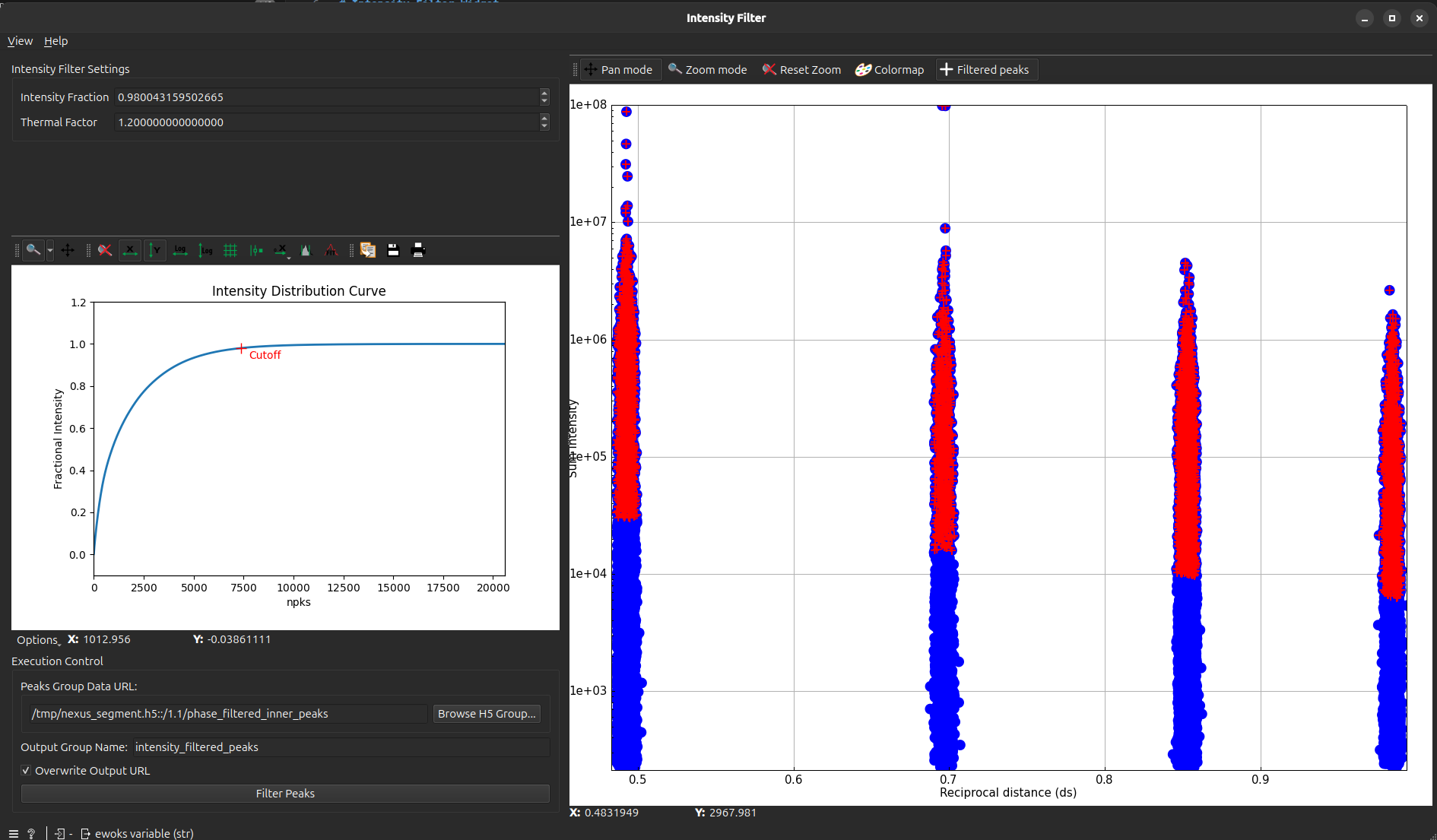
If you do run the task again, check Overwrite to overwrite to existing results or change the Output NeXus Group Name to save the peaks in a different group name (default: intensity_filtered_peaks).
Index filtering#
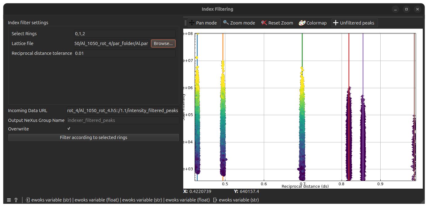
Double-click on the Index Filtering node, you will get the following window
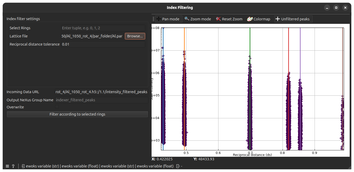
The peaks from Intensity Filtering will be displayed as crosses on the plot (as intensity of the peaks vs. the reciprocal distance).
In addition, the Lattice file field will be filled with the lattice used during the Lattice Filtering task so that lattice rings will also be shown on the plot (as colored lines).
In this widget, you will choose to keep only peaks for some of the diplayed rings. The rings are identified by their index starting from the left: the leftmost one is 0, the one after is 1, and so on.
Select rings by typing their indices as comma-separated values in the Select Rings field. The Reciprocal Distance Tolerance should be set to the same value set in Lattice Filtering (default: 0.01).
When clicking Filter according the selected rings, the results will be saved in the output file (default: indexer_filtered_peaks) and the plot will be updated as kept peaks will be appear as round markers.
As for previous filtering tasks, the output group name can be changed with the Output NeXus Group Name field and Overwrite can be checked to overwrite existing results when re-running the task.
Grid indexing#
Now that you have filtered the peaks to keep only those that are relevant, you can proceed to the task of generating grains, a process called indexing. This process uses a grid-based algorithm.
Initial Setup#
Double-click the Grid Indexing node to open the interface.
The Incoming Peaks tab displays the peaks passed from the previous filtering task (Index filtering). Before starting the process, configure the parameters in the control panel on the left:
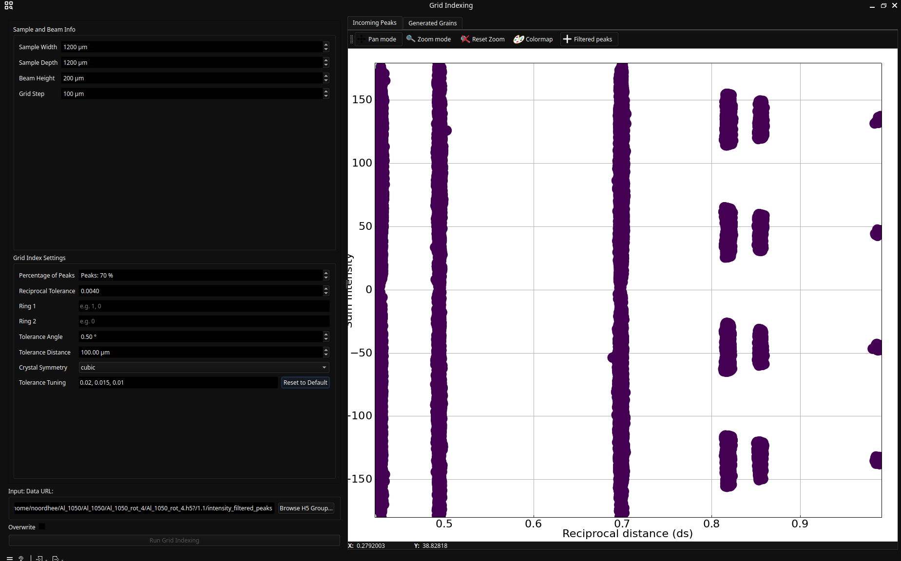
Sample and Beam Info: These parameters define the spatial grid for grain generation.
Dimensions: The grid should roughly match the illuminated area: Sample Width × Sample Depth × Beam Height.
Grid Step: This defines the minimum distance between grains.
Grid Index Settings: These control the generation algorithm. Hover over any parameter to view a tooltip with detailed information.
Ring 1 and Ring 2
The generation algorithm runs for every couple (r1,r2) with r1 the ring indices of Ring 1 and r2 the ring indices of Ring 2.
Example: if Ring 1 is 0, 1 and Ring 2 0, 1, the algorithm will run for the following couples: (0, 0), (0, 1), (1, 0) and (1, 1)
Also, do mind that Ring 2 should be a subset of Ring 1.
Execution and Monitoring#
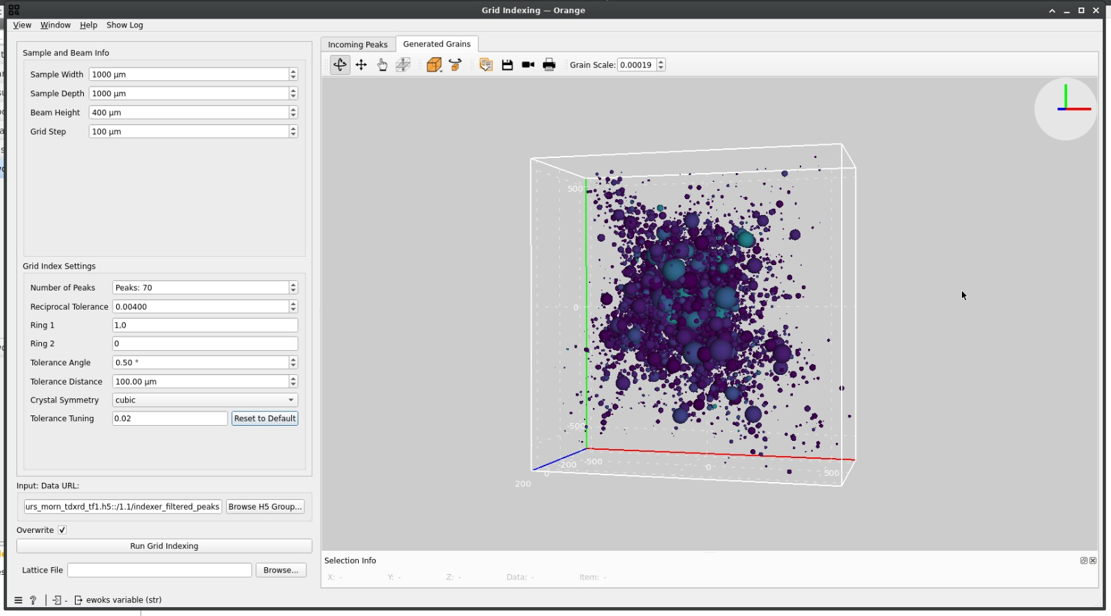
Once the parameters are set, click Run grid indexing. A window Grid Index Logs will pop-up and periodically update with grain statistics, grain positions and tolerance levels.
As the computation progresses, the Generated Grains tab on the right will update. The size of the grain will represent the mean intensity of the associated peaks while the color will represent the number of associated peaks.
When finished, the final list of grains is displayed in the 3D plot and saved in the output file’s scan group under grid_indexed_grains.
Use the 3D plot to explore the spatial distribution and orientation of the generated grains to evaluate the results (see next section) before moving to the final task.
Evaluating results#
Manual validation remains a crucial step in the 3DXRD data processing. You should have a rough idea of the crystallinity of your sample to evaluate if the number of found grains is right or not.
Note also that the spheres are approximations and not representative of the real grain shapes.
For example, the following picture shows a result where the generated grains are actually not realistic.
A good grain indexing usually shows fewer grains with a better repartition of the segmented peaks and less overlap:
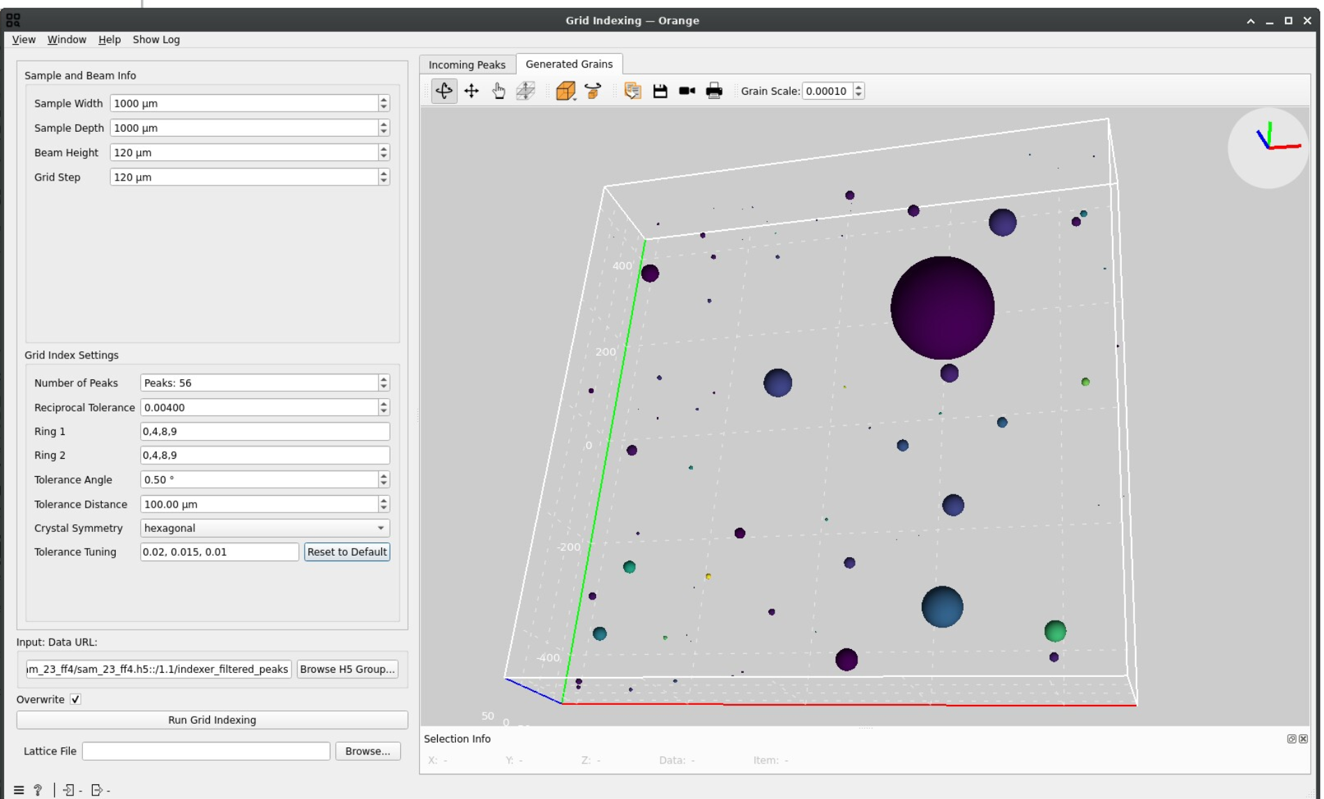
A high grain count may indicate noise being interpreted as real signal. Restarting from the Peaks segmentation step and making sure that no peaks are detected outside of diffraction spots may improve the indexing.
If grains overlap a lot, you may need to run the Grid Indexing task by choosing different, more well-behaved, rings for Ring 1 and Ring 2. Double-checking your geometry parameters by redoing a calibration and restarting from the Geometry transformation step may also be useful.
Info
A slight grain overlap may still be observed even with good parameters since the sphere representation of grain is only an approximation.
Troubleshooting#
If you receive an error stating the grain list is empty:
Try decreasing the Number of Peaks requirement so that more grains are retained during indexing.
Review your segmentation and filtering steps to ensure a sufficient number of peaks were passed through.
Verify that the lattice parameters used during filtering are correct for your material.
Refine grain mapping#
The objective of this final task is to iteratively refine the crystallographic and spatial parameters of the grains obtained during the Grid Indexing stage. This ensures higher accuracy in the final reconstructed grain map.
Setup#
Double-click the Refine Grain Mapping node to open the interface.
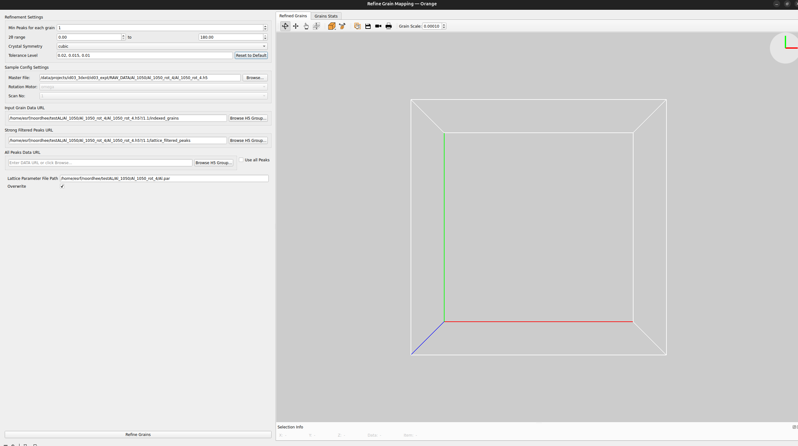
In the Refinement settings panel, you can configure the optimization algorithm. As with previous widgets, hover over any parameter for a detailed tooltip.
A very important parameter is the Tolerances field where multiple tolerances must be given, separated by commas. The iterative refinement algorithm will go through each tolerance subsequently to optimize the grain orientations and positions. In other words, the number of tolerances represent the number of iterations of the algorithm and the tolerances should be decreasing to refine grain parameters further and further.
Execution#
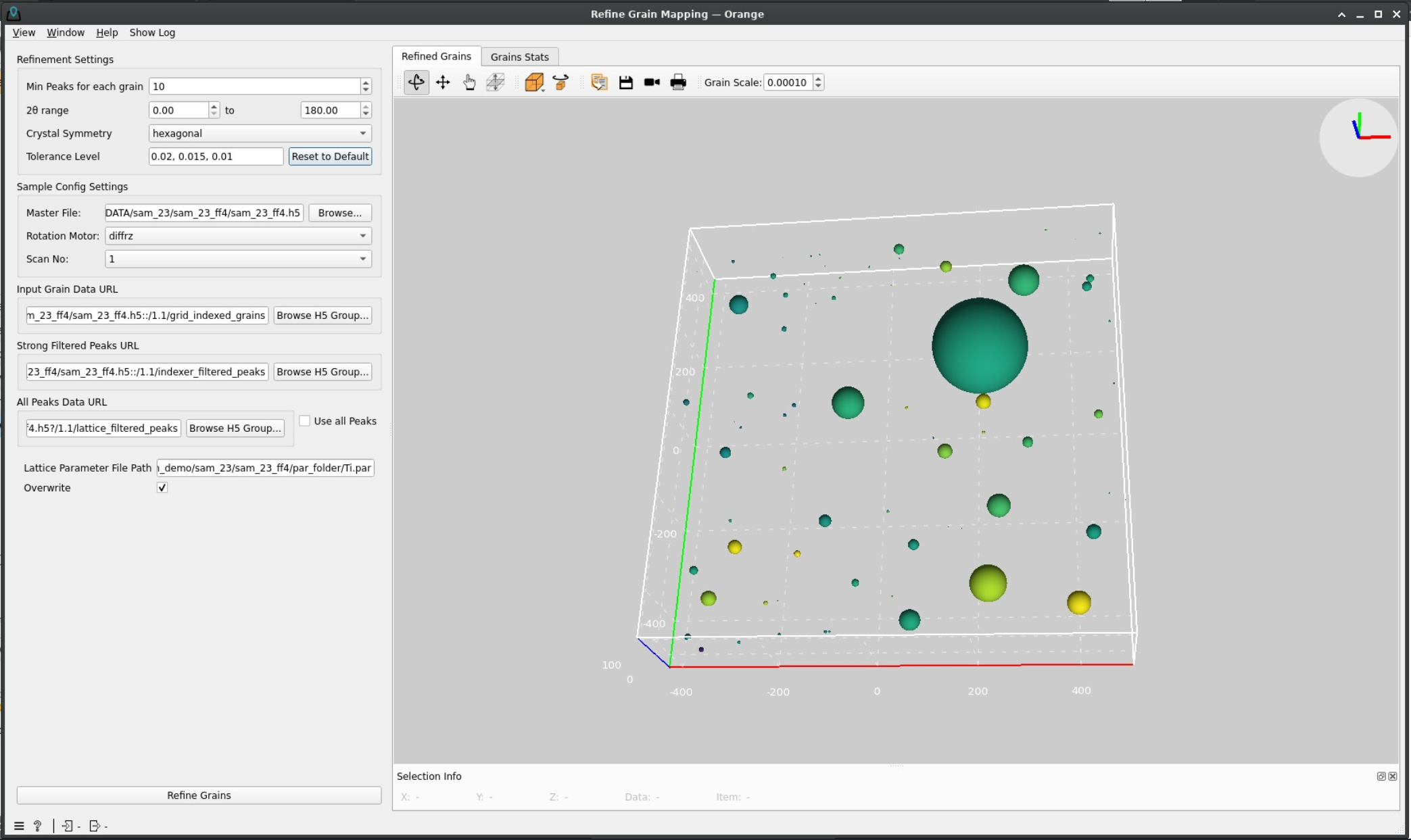
Once your parameters are configured, double-click on Refine Grain Mapping.
During the process, a pop-up window will track the progress of the iterations and the 3D plot and statistics will update periodically as the refined grain parameters are computed.
Once the computation finishes, the plot on the right will be updated one last time with the refined grains and these will be saved in the scan group of the output file under make_map_grains.
Final words#
You have now reached the end of the Ewoks3DXRD workflow tutorial! You should now have an HDF5 file containing all the results, looking like the one below (viewed here with myHDF5)
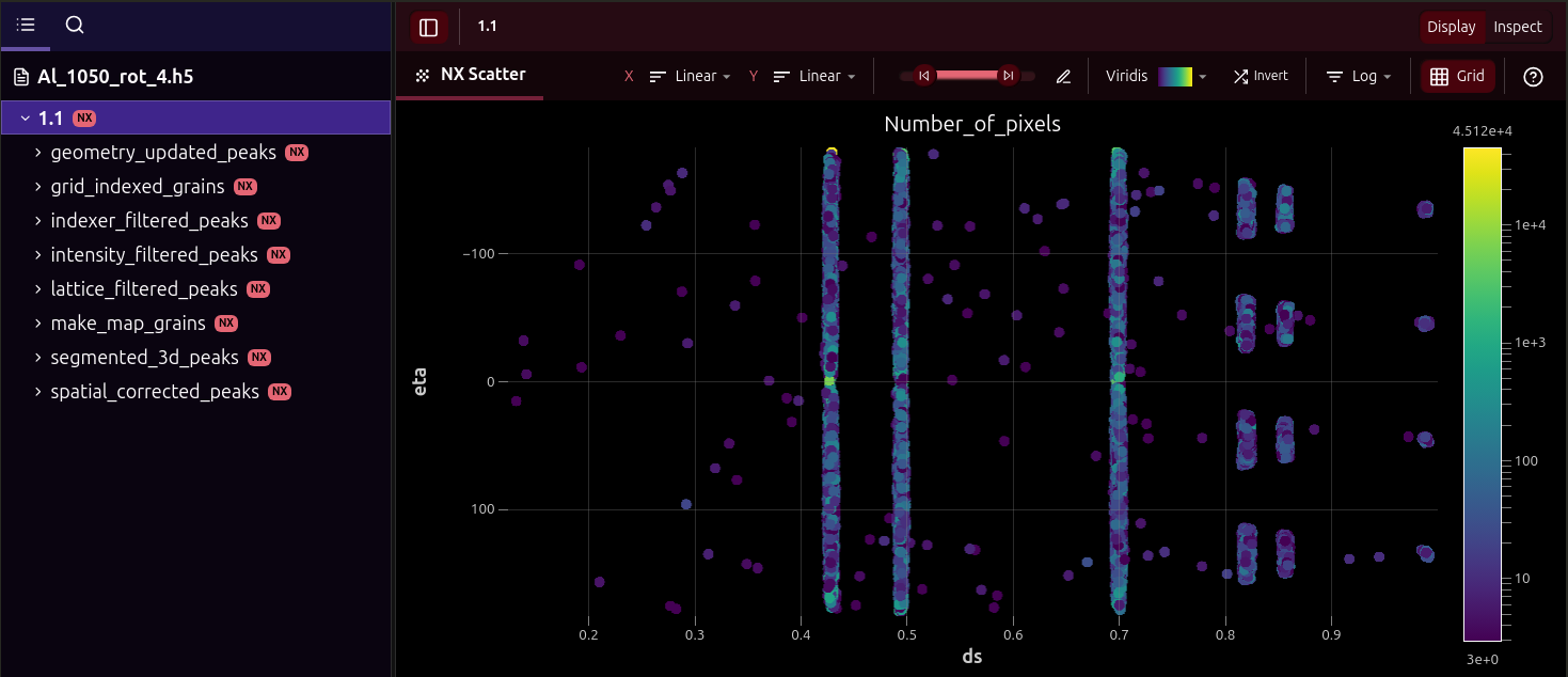
You can inspect the results outside of the workflow by using the CLI ewoks3dxrd-grain-vis
ewoks3dxrd-grain-vis <path_to_output_file> -e <scan_number (default: 1.1)>
See the Visualization page for more info on this.
Processing 3DXRD data is a complex task and there is a lot of information left out from this tutorial for the sake of simplicity. Dedicated sections will be created in the future for deeper dives on certain operations and concepts.
In the mean time, you can still open an issue on our Gitlab repository if you encountered any issue during this tutorial or would like to provide feedback.
Thanks for reading!